Q Learning

In my quest to learn more about reinforcement learning, I’ve come to Q learning. We’ll be implementing it on the Taxi-v3 environment from OpenAI’s gym. In this environment, a virtual self-driving taxi takes virtual passengers to virtual dropoff points, and our goal is to teach the taxi how to do this well.

Here’s the taxi in action (slowed down so it’s possible to see what’s going on):

Q learning is so-called due to the Q function, \(Q(s, a)\) which takes in a state and an action and returns a prediction of future reward. Because Taxi-v3 has a small, discrete number of both states and actions, it’ll be easy for us to implement Q as a table, mapping state-action pairs to numbers. There is also a “deep” variant of the algorithm, using a neural network to approximate the Q function, which won’t be covered here.

After importing useful libraries, we can set up the environment with env = gym.make('Taxi-v3')

The Q table

There are 500 possible states for this little world to be in, and 6 actions the taxi can take. Therefore, a table with 3000 entries will do the trick just fine for implementing \(Q\).

q_table = np.zeros(
    (env.observation_space.n, env.action_space.n))

In environments with either non-discrete actions/states or way too many actions/states to reasonably fit in a table, a different approach would be warranted.

Action Selection

Learning requires a bit of random exploration, to make sure that we’re testing out new actions and finding whether they perform better than what we would have done anyways. However, there’s a tradeoff here as the more we explore, the less we get to exploit our known preferred actions. Letting exploration_chance be the probability that we explore vs. exploit known actions, we have

if random.random() < exploration_chance:
    action = env.action_space.sample()
else:
    action = np.argmax(q_table[state])

However, as I’ll mention later, likely due to the sheer number of episodes acting as a good-enough randomizer themselves, exploration wasn’t actually very important in the context of this specific problem.

Updating the table

The most important step within the overall algorithm consists of making updates to that table.

The learning/update step requires updating the cell in the table referring to the current action-state pair. It’s given by a formula incorporating the learning rate and discount factor hyperparameters and updates the old value based on an expectation of future reward.

This image¹ captures the meaning of the update step better than I could; I wish more equations were annotated in this way:

In code, this translates to

old_value = q_table[state, action]
q_table[state, action] =
    old_value + learning_rate * (reward + discount_factor *
    np.max(q_table[observation] - old_value))

Hyperparameters

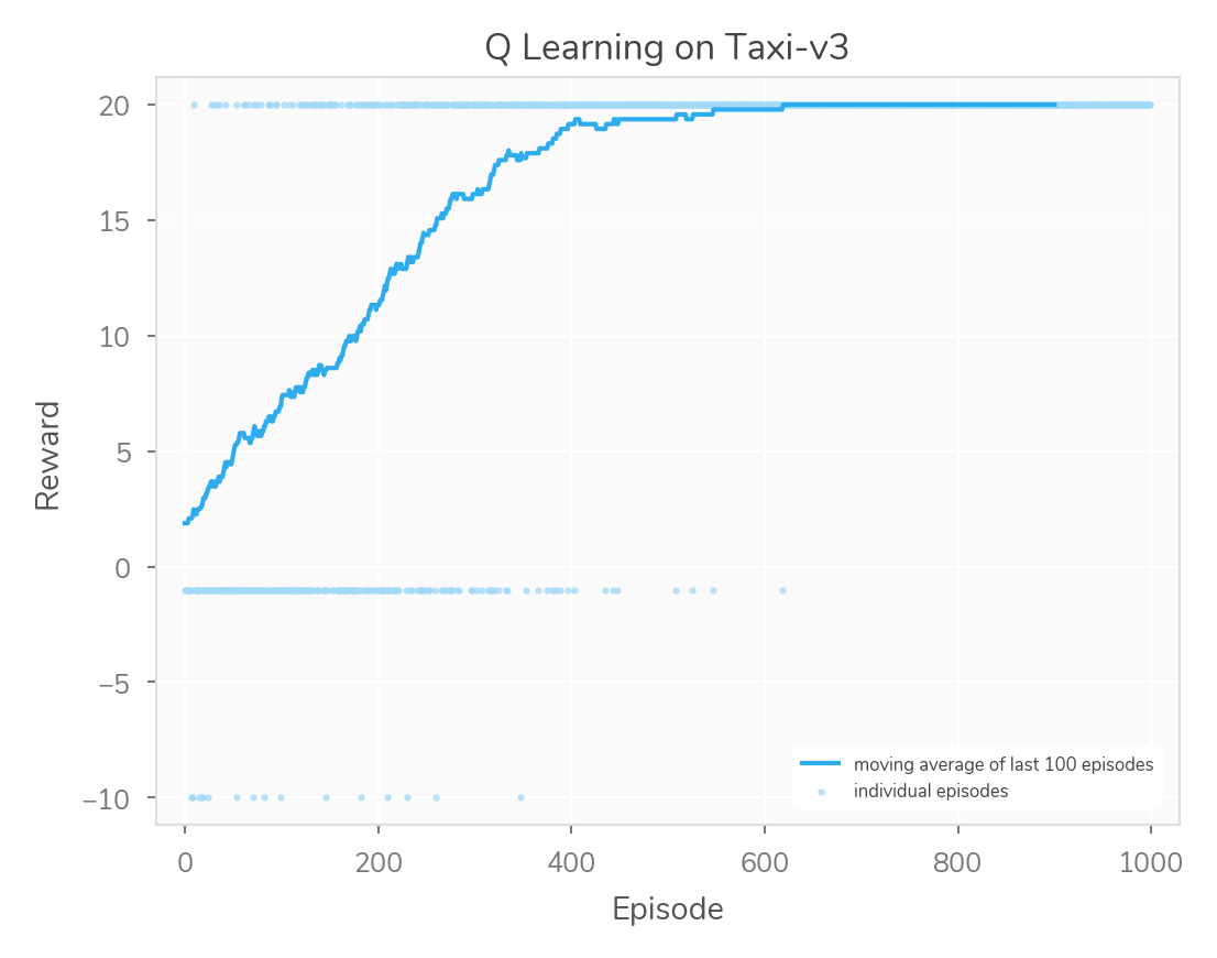
I ended up finding that these worked fine for my case, and didn’t bother with metalearning the hyperparameters themselves (e.g. with grid search).

num_episodes = 1000
learning_rate = 0.1
discount_factor = 0.75
exploration_chance = 0.1

This set of numbers led to a nice quick learning curve which was extremely stable once it got through a few hundred episodes:

The exploration chance was probably the most fun parameter to play with, here it is at 90%:

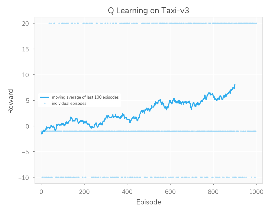
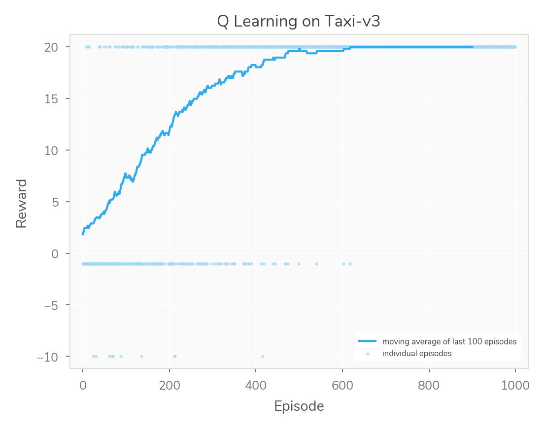
Obviously, learning is slower when we act super erratically. However, I found it interesting that an exploration chance of 0% didn’t seem to perform too badly here. I assume it’s more important to explore (vs. exploit) in other, more-complicated contexts. Here’s the learning curve for a 0% exploration rate.

The code from this example is on GitHub