Vanilla Policy Gradient

Background

Vanilla Policy Gradient (VPG) is—as the name “vanilla” suggests—a basic way to get started with policy gradient algorithms. It’s also sometimes called “REINFORCE”.

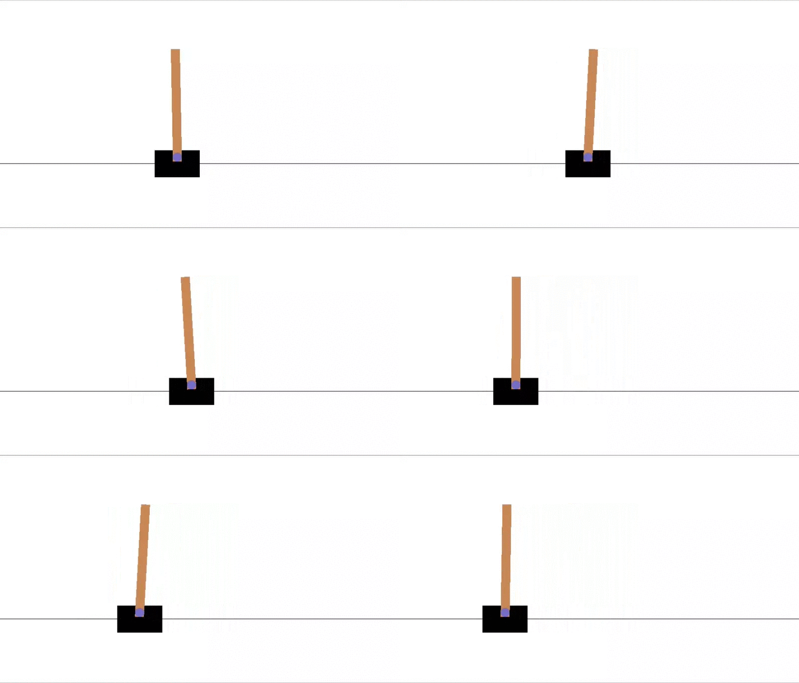
We’ll be testing out our implementation in the CartPole environment. In this environment, our job is to balance a pole on top of a cart. At each step, we can either move the cart left or right. A moderately well-trained VPG CartPole agent looks like this in action:

Math

We want to learn some policy \(\pi : S \rightarrow A\) mapping from states to actions¹. In our case, we’ll want to frame this more like a probability \(P(A | S, \theta)\) indicating the probability we take action \(A\) given current state \(S\) and initial parameters \(\theta\). Some resources more formally state this as \(\pi : S \rightarrow \Delta(A)\), with \(\Delta(A)\) meaning the probability simplex over \(A\)². (“Probability simplex” here roughly means that we have a mathy way to convert to a bunch of non-negative real numbers that sum to one.)

To simplify, we just want our policy to look something like [0.1, 0.7, ...], meaning our policy is that we should have a 10% probability of taking the first action, 70% of taking the second action, etc. We have a probability distribution over which action we should take.

We use softmax: \(\sigma(x)_i = \frac{e^{x_i}}{\sum_{j=1}^{k}e^{x_j}}\) for the output layer in the neural network, to convert into action selection probabilities. It’s a handy function to know about when you want to work with probabilities: softmax converts each component in some vector into a number between zero and one, and all of the components add up to one.

Along with a definition of a policy on which action to take for each state, we need a loss function that helps guide us in updating our weights, i.e. actually learning from an episode. Our discounted reward is the sum over all timesteps in an episode of the per-state reward, multiplied with a discount factor \(\gamma\) that increases exponentially with time. Calling the current time \(t\), and the reward at that time \(R_t\) we get a total discounted reward of \(\sum_{t} \gamma^{t} R_t\).

Using this discounted reward \(G_t\), we can multiply the rewards by the log probabilities³ that we touch each action given some state, averaged over time. Our loss then take the form \(-\frac{1}{t} \sum_t \ln (G_t \pi_t)\). We descend along the gradient to get the new policy, with updates learned.

Code

Full code is available in the github repo

A sketch of how policy gradient works in pseudocode might look like this:

class PolicyEstimator():
    def __init__(self, env):
        # build the neural network structure
        self.network = ...

    def predict(self, observation):
        # use the network to provide probability distribution
        # over actions
        return self.network(observation)

def vanilla_policy_gradient(env, estimator)
    # for CartPole, we have two actions: move either left
    # or right
    action_space = [0, 1]

    for episode in episodes:

        while True:

            action_probs = estimator.predict(observation)

            # choose an action, weighted towards those with
            # higher probability
            action = choice(action_probs, p=action_probs)

            observation, reward, done, info = env.step(action)

            # keep track of things
            observations += observation
            rewards += reward

            if done:
                # apply discounting to rewards
                discounted_rewards = ...

                total_rewards += sum(rewards)

                if end_of_batch:
                    # calculate loss with log probabilities
                    loss = ...

                    backprop()
                    optimize()

                print(episode, reward)

                # this is optional, but you can break out
                # once your reward reaches a certain amount
                if reward > early_exit_reward_amount:
                    return total_rewards
                
                # move on to next episode
                break

    return total_rewards

def main():
    env = gym.make(environment_name)
    rewards = vanilla_policy_gradient(env,
        PolicyEstimator(env))
    plot(rewards)

The actual code isn’t terribly much more complicated than this. It does have to do a little bit of extra bookkeeping, and deal with semi-finicky things like getting tensor shapes correct. However, this should hopefully translate fairly directly from a general outline into runnable code.

Output

While running, the code provided should spit out lines like this every few seconds:

average of last 100 rewards as of episode 0: 15.00
average of last 100 rewards as of episode 100: 27.20
average of last 100 rewards as of episode 200: 35.73

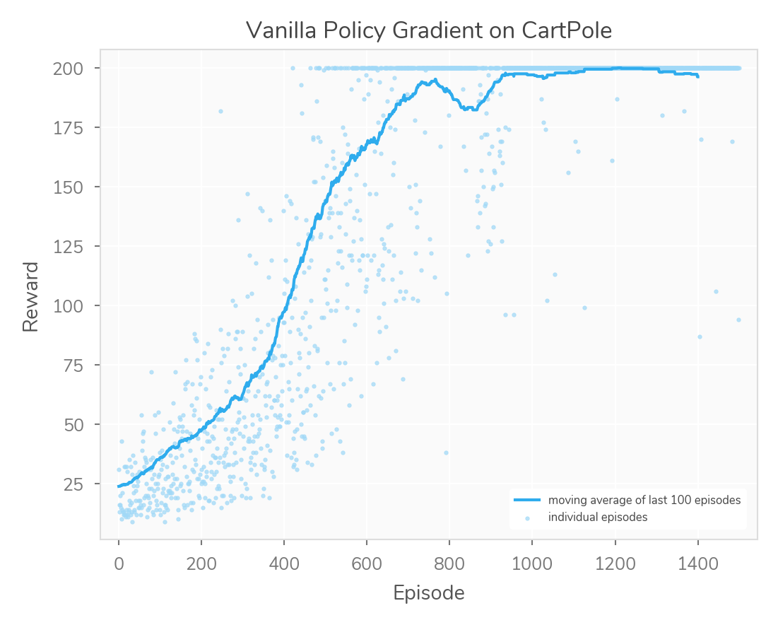
You might notice that the reward hops around a bit, sometimes decreasing instead of increasing. This happens especially often once we reach the later stages of training, and have already had some episodes attaining the maximum reward. Because the reward is capped, there isn’t much left to do once you reach the cap, but the algorithm will still search around—typically dipping down for a while before coming back up.

Here’s a final output graph of a training session:

Notice that this session has one of those dips. Reward doesn’t monotonically increase. Also, notice that VPG is relatively noisy. There are ways to fix some of these issues, but this is “vanilla” for a reason. It’s a basic algorithm, easy to implement, but of course we can do better by taking advantage of more-advanced ideas.

VPG should provide a decent skeleton for building further policy-learning algorithms, and for learning more about reinforcement learning in general.