Guessing a Function

Let’s play a game. I’m thinking of a continuous mathematical function defined over the domain between zero and one, with output values ranging between zero and one. Your job is to figure it out in as few guesses as possible.

Of course, the function I’m thinking of could be extremely complex, so we’ll need to add some leniency. Let’s say that your guess is “correct” if it “loses” by less than \(0.05\). We’ll define this loss number in a second (it’s just a mathematical function of your guess). For simplicity, we’ll call my function \(f\) and your guessed function \(g\).

First, do you have any hope at all of approximating any function I come up with? The Weierstrass approximation theorem tells us that this can be done to arbitrary levels of precision using polynomials. So now all you need is a procedure for generating polynomials that better approximate my function at each step, and you’re guaranteed to find my function eventually.

Here’s an example. In all these graphs, the bottom left corner is at \((0, 0)\) and the top right corner is at \((1, 1)\).

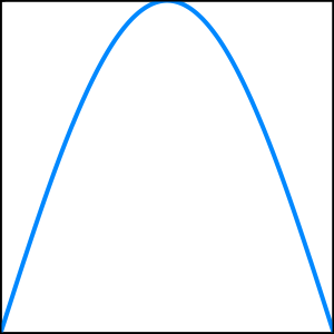
The function I’m thinking of, \(f\), is the blue line. I won’t tell you what it is yet, because that would ruin the game! But it’s clearly continuous, defined between zero and one, and guessable.

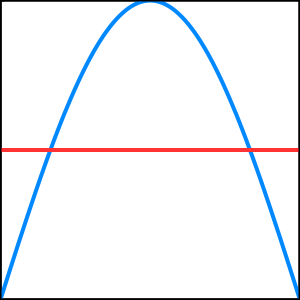
You should try to get your bearings now. One possible initial guess might be the constant function \(g_1 = \frac{1}{2}\). Conveniently, this is a polynomial (of order zero) that is at most \(0.5\) away from \(f\) at every point. Obviously this won’t be a very good guess, but it will help us find out how far away from my arbitrary function you are. A plot of \(f\) and \(g\) now looks like this:

Although in our guessing game you don’t have access to this information, we can also plot the absolute value of the difference between the two functions:

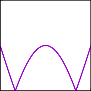
It’ll be hard for you to generate a second guess better than your first guess without a bit of additional information. I’ll take the difference plot above and give you its integral over the domain \([0, 1]\). This number is the amount your current guess lost by, which we can call the “loss”.

To put it mathematically, I’ll give you \(\int_0^1 \left| f - g \right|\), which in this case is just \(\int_0^1 \left| f - \frac{1}{2} \right|\). The loss number I give back to you for your guess \(g_1 = \frac{1}{2}\) is \(0.2994\). It’s not yet less than \(0.05\), so you should guess again!

You take several more guesses, gradually learning more and more about the general shape of \(f\). I’m eliding most of the hard work from this post, involving a lot of guessing and logic based on what you’ve previously learned about \(f\), but let’s assume that eventually you start honing in on a reasonable shape for \(f\) and really just need to adjust some parameters until your guesses are close enough that you win the game.

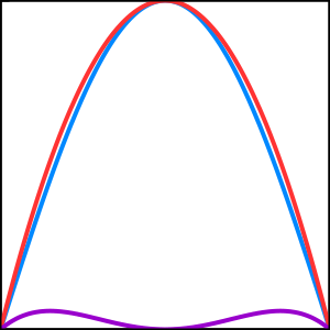
Your next guess might be \(g_n = -2(x-\frac{1}{2})^2 + 1\). Here’s what that looks like, along with my function \(f\) and the loss function \(L\):

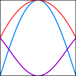
With a loss of \(0.1967\), this isn’t quite good enough. Skipping forward quite a bit, you start learning which parameters tend to decrease the loss when pushed in the right direction. Eventually, you’re able to update your guess to \(g_f = -4(x-\frac{1}{2})^2 + 1\).

The loss here is \(0.0301\). Finally you’ve succeeded!

The Point

There are a few interesting pieces to note here. Your final function \(g_f\) is clearly not the same as the function \(f\), because the loss isn’t zero! However, even if the loss were zero, there’s no guarantee that you’ve actually found the same function I was thinking of. What if the two functions are the same between \(0\) and \(1\) but have different behavior outside that box?

We also haven’t clearly outlined a procedure for discovering better function approximations. Although the function, the guess, and the loss are all clearly defined, there’s still quite a bit of tweaking and guesswork that goes into your procedure for finding the same function as I was thinking of. Just because we can approximate any function meeting our requirements arbitrarily well, doesn’t mean that there’s a straightforward procedure for constructing those kinds of functions.

Another interesting point to note is the difference in information due to dimensionality constraints. What I mean here is that given the loss function itself, which exists in two dimensions, we can instantly find \(f\) from \(g\) and the loss by simply “making up” the loss and adding it back into \(g\) to get \(f\). It’s only because the loss is a single scalar that we have difficulty fully using the information it gives us.

If the loss were any encoding that accounts for the full range we care about, then as long as we know that encoding we’d be able to trivially reconstruct \(f\). However, even knowing the exact encoding of the loss as it currently is (the integral of the absolute value of the difference), there is some information we can’t come up with.

Bonus points, by the way, for guessing the actual function \(f\):