Stanley Cup Probabilities

While watching the Stanley Cup Finals recently, we heard the announcers mention something interesting: historically, 75% of teams who win the first game of the series go on to win the overall series.

There might be many reasons for this, including team psychology, ordering of home and away games, the fact the first game might be revealing underlying information about which team is truly better, and so on. However there’s one possible reason that I’d like to focus on here: if you win the first game, you’re one game closer than your opponent to winning the series (three games away instead of four). Even if the teams are perfectly evenly matched, and further game outcomes are random, there’s still an advantage.

So, what’s the probability that the winner of the first game wins the series, assuming each subsequent game is like a perfect coin flip? We’ll take a few different approaches to solving this problem—an approximate Monte Carlo simulation, a fully exact enumeration, and doing combinatorial math.

Approximate Monte Carlo simulation

One easy way to play with this situation is to code up a simple randomized simulation and see what happens when we run it a large number of times. We can simulate a single game as a bit decided by a coin flip: either 0 or 1.

import random

def simulate_game():
    return random.choice('01')

We’ll select 0 to be the team that wins the first game. Given that, we can simulate a full series like this:

def simulate_series():
    so_far = '0'
    for _ in range(6):
        so_far += simulate_game()
        if so_far.count('0') >= 4:
            return '0'
        elif so_far.count('1') >= 4:
            return '1'

The first team to reach four wins will win the overall series. Now all that’s left to do is run this single-series simulation a bunch of times, and count up the times the team who won the first game wins the overall series.

num_simulations = 1000000
wins0 = 0

for i in range(num_simulations):
    if simulate_series() == '0':
        wins0 += 1

print(wins0 / num_simulations)

This is really quite an easy way to get a quick answer, and it’s not super prone to error since each step is very simple to reason about. However, it can only give us an approximation, not an exact result. We tend to get a final answer somewhere around 65.6%.

Exact enumeration

Stanley Cup playoff games are structured as a best-of-seven series of games. We can model a series of games as a bitstring with 0 representing the first team winning a game, and 1 representing a win for the second team. Some possible ways a series might turn out are:

Notice that a series is valid if and only if there are either exactly four 0s or exactly four 1s, and the series doesn’t continue after a team has won four games. This implies a bunch of other facts, like the minimum number of games played being four, and the maximum being seven.

We can write a function accept that takes a bitstring (of length between four and seven) and returns a boolean, for whether that bitstring is valid. As well as accepting the bitstrings above, we should reject these ones:

My girlfriend (who’s currently learning Python) offered to do the task of writing accept. Here’s what she came up with:

def accept(bitstring):
   for i in range(3, len(bitstring)):
       substring = bitstring[:i+1]
       if substring.count('0') == 4 or substring.count('1') == 4:
           return len(substring) == len(bitstring)

Because there are \(2^4 + 2^5 + 2^6 + 2^7 = 240\) possible bitstrings with lengths between four and seven inclusive, we know there’s a pretty small upper bound on the number of possible series. We already have accept, so it’s not too hard to create a list of all the valid possibilities.

possibilities = []
for exp in range(4, 8):
    for n in range(2 ** exp):
        s = format(n, f'#0{exp + 2}b')[2:]
        if accept(s):
            possibilities.append(s)
print(len(possibilities))

From this, we find that there are 70 possible valid series of playoff games. Of course, we only want to count the playoffs where one specific team won the first game. As you would expect, there are 35 playoffs (half of 70) where team 0 won the first game.

for exp in range(4, 8):
    for n in range(2 ** exp):
        s = format(n, f'#0{exp + 2}b')[2:]
        if s[0] == '0':
            if accept(s):
                print(winner(s), s)

Here are all of the possible series with a first game won by team 0, with the winner of the series listed in the first column.

We’ve made a good amount of progress, since now we know the very limited set of ways that a series can play out. However, it’s important to note that this still doesn’t tell us the relative likelihoods of each series. To see why, consider this decision tree for a best-of-three series:

The labels on each edge represent the probability mass flowing into the node below as a percentage of the whole. To find out the chance of any particular series, we can look at the label of the edge just above it. In this case, the winners are:

0 00
0 010
1 011

Because the series 00 has 50% probability of showing up (i.e. has more weight than the other two scenarios), the chance that team 0 wins a best-of-three series given they win the first game is actually 75%.

Going along with our theme of enumeration, let’s see a full decision tree for a best-of-seven series. (Click to open full-size image in a new tab):

Let’s focus in on a small slice of that giant tree. Just like above, the fractions on edges indicate the probability of hitting a node out of the total. Dotted nodes represent (prefixes of) series that haven’t finished yet. Playoffs won by team 0 have red outlines, and playoffs won by team 1 are outlined in blue.

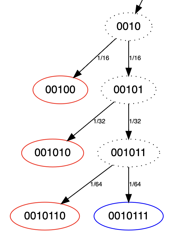
Now, all we have to do is add up the probabilities going into each red node….

Our final answer is that \(\frac{21}{32} = 65.625\%\) of series where team 0 wins the first game are won by team 0.

Combinatorics

The fact that the first game is won by team 0 is a given.

There is only one way to end the series in four games: 0000. The chances of this happening are the chances of getting three zeros in a row (since the first is a given).

\[\left(\frac{1}{2}\right)^3\]

Another important thing to note is that if team 0 wins the series, this implies they won the last game (as well as the first). This means we’re limited to only placing 1s in the middle. We should count the number of ways 0 can win any given series length, and multiply by the probability of getting a bitstring that long. The number of possible series here is the same as the number of ways to place 1s in the “available slots”. For a four-game series, this boils down to:

\[\left(\frac{1}{2}\right)^3 {2 \choose 0} = \frac{1}{8}\]

The \({2 \choose 0}\) means we’re choosing how to place zero 1s in two slots, and the \(\frac{1}{8}\) is the same as before (one over two to the number of decisive games played).

For a five-game series, we have:

\[\left(\frac{1}{2}\right)^4 {3 \choose 1} = \frac{3}{16}\]

This is because we have three slots for games (in between the given 0 games at the beginning and the end) and team 1 can only win one of them.

The six-game and seven-game playoffs will follow similar reasoning:

\[\left(\frac{1}{2}\right)^5 {4 \choose 2} = \frac{3}{16}\]

\[\left(\frac{1}{2}\right)^6 {5 \choose 3} = \frac{5}{32}\]

We can express the overall chances that team 0 wins with this formula (where \(n\) is the number of games won by team 1):

\[\sum_{n=0}^{3} \left(\frac{1}{2}\right)^{n+3} {n + 2 \choose n} = \frac{21}{32}\]

Parameterization

One final note: if we wanted to, we could parameterize each of our solutions with a win probability that isn’t exactly 50%. In the simulation approach, we would change simulate_game to return random wins according to the new win probability. In the enumeration, we label edges differently based on whether they were won by team 0 or team 1, and continue to multiply probabilities as before. And finally, we can plug in a fraction other than \(\frac{1}{2}\) to our combinatorial formula.