Navigating with Dijkstra

Have you ever been stranded on the side of the highway, trying to navigate across the country, when all you had available was a geojson file of the US freeway network, and a specialized computer that could only run Blender?

Well to be honest…me neither. However, every once in a while, I like to attempt a small programming project that’s heavy on data structures and algorithms. It reminds me of school, I guess. We’ll be using this dataset of the US Freeway System, Dijkstra’s algorithm, and a bunch of different data structures to write a reasonably efficient tiny routefinding application.

Full code for this post can be found in this gist.

I think I’ve historically underused Blender for math-to-visualization applications like plotting points, highlighting edges, or (in this case) drawing planar graphs in space. So, let’s try using it. We’ll want to import bpy and run this script from Blender’s Scripting tab—in fact, we could do this entire project purely inside Blender. However, Blender’s text editor isn’t great, so I recommend using the external editor of your choice, and loading that script file into Blender like this:

filename = "dijkstra_roadmap.py"
exec(compile(open(filename).read(), filename, 'exec'))

To get our script started, we’ll import a bunch of data structure libraries and ways to manipulate them.

import bpy
import collections
import json
import math
import queue

Conveniently, there’s a single longitude that cleanly splits Alaska and Hawaii off from the continental road network. We’ll use that to only focus on the continental US.

westernmost_longitude = -130

We can define a distance function between two coordinates a and b. Here, we’re using the simple Euclidean distance, although this ignores things like the curvature of the earth, map projection, and the little bit of distance added by changes in altitude. Making this a function at least means it remains open to being fixed in the future.

def distance(a, b):
    ax, ay = a
    bx, by = b
    return math.sqrt((ax - bx)**2 + (ay - by)**2)

The first big step isn’t tricky in terms of algorithms, but it does introduce several data structures that we’ll be using. coords is a list of (x, y) (or longitude/latitude) coordinates. As we build this list, the index of each element added is stored in indices, and the other direction (from index to coordinate) is stored in reverse_indices.

Together, indices and reverse_indices represent a bimap—a two-directional map that can go from coordinate to index or vice versa. We don’t need to use an “actual” bimap data structure simply because using two dictionaries is very easy—especially when we won’t be updating the bimap after initially populating it. These maps will be handy for efficient conversions between coordinates and indices later. Finally, edges is a list of (index, index) pairs, indicating which vertices in the graph are connected by an edge.

Note that this is where we exclude coordinates that are too far west—we won’t need to think about them for the rest of the project. We also transform both MultiLineString and LineString into a list of lines, so we can easily map over all the geometry using the same code.

coords = []
edges = []
indices = {}
reverse_indices = {}

with open('USA_Freeway_System.json') as f:
    data = json.load(f)

for feature in data['features']:
    feature_lines = []
    if feature['geometry']['type'] == 'LineString':
        feature_lines = [feature['geometry']['coordinates']]
    elif feature['geometry']['type'] == 'MultiLineString':
        feature_lines = feature['geometry']['coordinates']

    for line in feature_lines:
       for [x, y] in line:
           # ignore alaska and hawaii
           if x > westernmost_longitude:
               indices[(x, y)] = len(coords)
               reverse_indices[len(coords)] = (x, y)
               coords.append((x, y))
       for a, b in zip(line, line[1:]):
           ax, ay = a
           bx, by = b
           if ax > westernmost_longitude and bx > westernmost_longitude:
               edges.append((indices[tuple(a)], indices[tuple(b)]))

print('num coords:', len(coords))

After ingesting this data, we see

num coords: 255307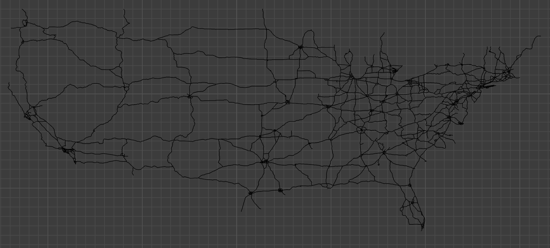

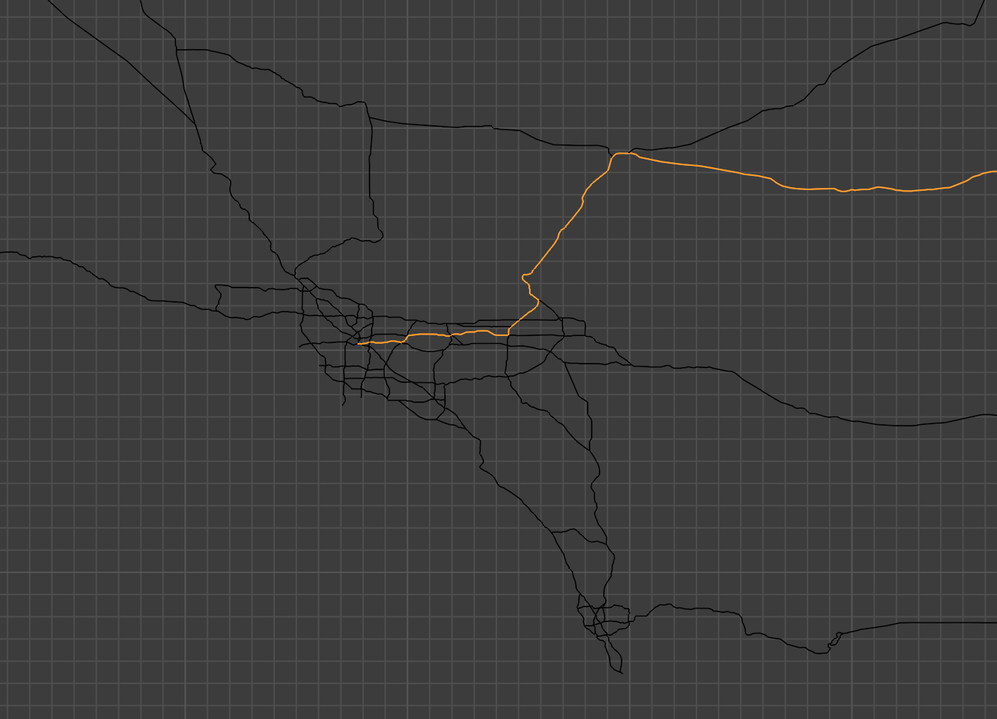
To do our routefinding, we need a start point and end point for our route. We’ll start in the southwest (near downtown LA) and end in the northeast (in Maine). I’ve selected two points that are already in our list of coordinates, although it’d be easy enough to account for arbitrary data entry by simply adjusting to use the nearest coordinate that’s actually in the list. (We could use a quadtree data structure to do this efficiently.)

start = (-118.226138727415, 34.0285571022828)
end = (-67.7811927273625, 46.1339890992705)

Next up is another fairly straightforward algorithm to populate a useful data structure. We’re using defaultdict—one of my favorite Python datatypes—that will store the set of neighboring indices for each point (at its index). Now we can quickly get all the neighboring vertices of any vertex in the graph.

neighbors = collections.defaultdict(set)
for a, b in edges:
    neighbors[reverse_indices[a]].add(reverse_indices[b])
    neighbors[reverse_indices[b]].add(reverse_indices[a])

Several parts of the map have pretty significant complexity—usually around cities. A prepopulated data structure for neighboring vertices avoids extra traversal of the graph.

Here’s the actual pathfinding code. We’re using a fairly standard implementation of Dijkstra’s algorithm using a min priority queue (ordered by distance). We also have a map from coordinates to their distances along any route, that starts out as a map from each coordinate to infinity. While searching, if we find a shorter path we add that new (lower) distance as the priority for that vertex. At the very end, we convert from prev’s singly-linked list of previous coordinates along our route to a stack s (here just prepending to a Python list). We now have the list of coordinates from start all the way through to end.

dist = {}
prev = {}
remaining = queue.PriorityQueue()

for coord in coords:
    dist[coord] = math.inf
    prev[coord] = None

dist[start] = 0
remaining.put((dist[start], start))

while not remaining.empty():
    _, u = remaining.get(False)

    if u == end:
        break

    for v in neighbors[u]:
        alt = dist[u] + distance(u, v)
        if alt < dist[v]:
            dist[v] = alt
            prev[v] = u
            remaining.put((alt, v))

s = []
u = end
while prev[u]:
    if u == start:
        break
    s = [u] + s
    u = prev[u]

With s full of coordinates, we can convert into a list of edges.

pathedges = []
for a, b in zip(s, s[1:]):
    pathedges.append((indices[a], indices[b]))

Finally, we’ll want to write out our data to Blender, which can handle representing it. We provide two lists of edges to generate_mesh—one for the base map with all freeways, and a second for just the edges on the route our algorithm found.

def generate_mesh(name, edges):
    mesh = bpy.data.meshes.new(name + "mesh")
    obj = bpy.data.objects.new(name, mesh)
    mesh.from_pydata([(x, y, 0) for (x, y) in coords], edges, [])
    mesh.update()
    bpy.context.collection.objects.link(obj)

generate_mesh('basemap', edges)
generate_mesh('path', pathedges)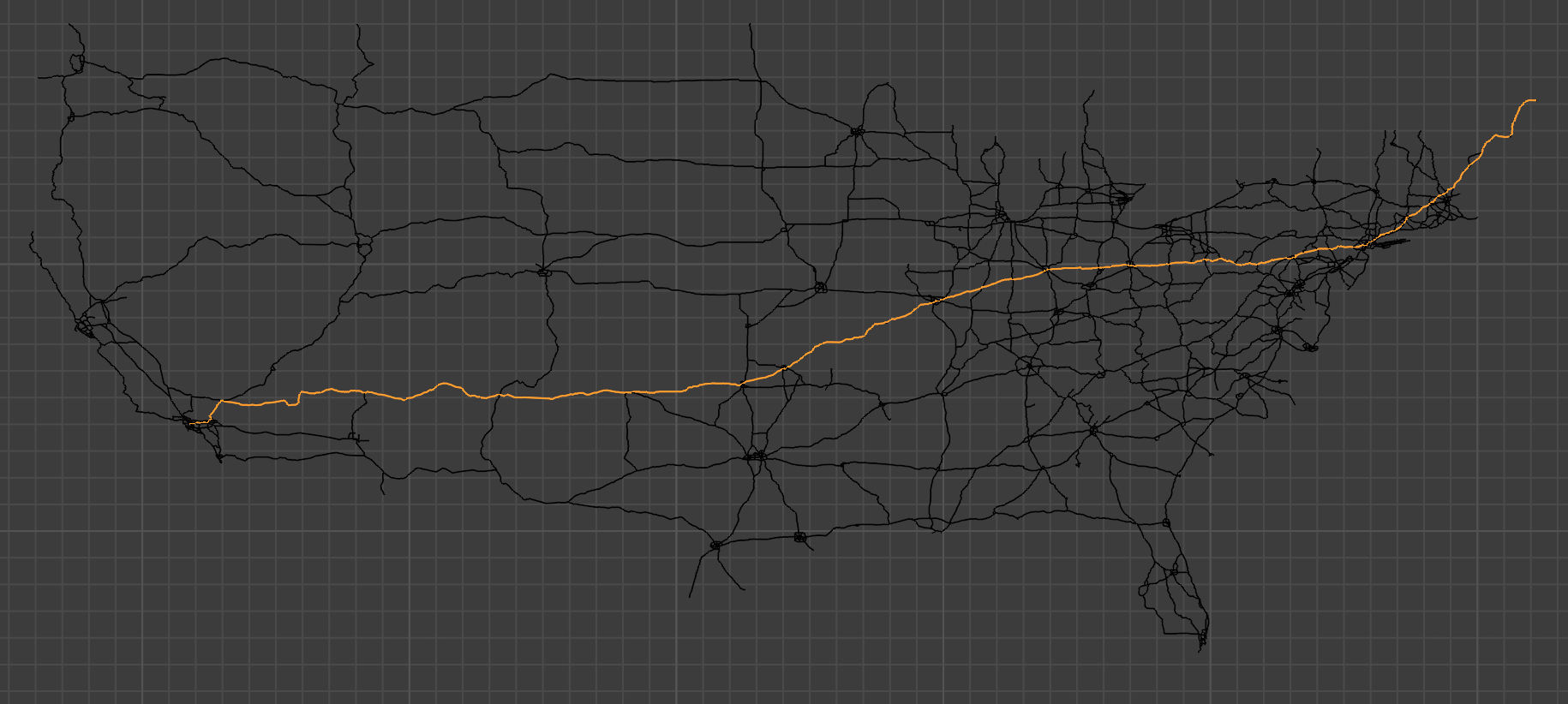

Of course, there are further optimizations and adjustments we could do to make our little route finder a better application. It’s possible to take into account factors like speed limits, real-time road closures, and so on in a real mapping app.

Even without extra information, we can make our pathfinding faster by…you guessed it, using different data structures. Consider the three segments of highway below, between cities.

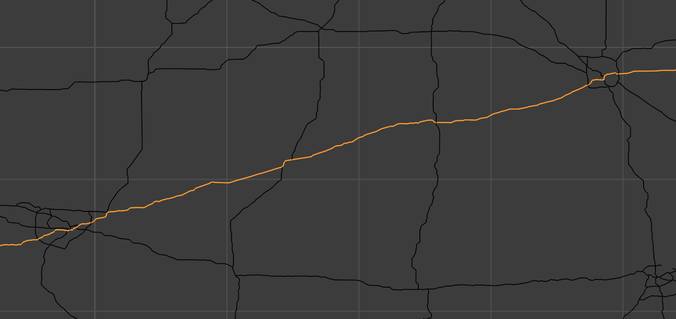
Instead of representing these roads as lists of all their coordinates, including the little twists and turns along them, we could instead represent them as single edges along with a distance number that captures those smaller turns. This leads to a huge simplification in our map’s internal representation. From this code…

counts = collections.defaultdict(int)
for neighbor_set in neighbors.values():
    counts[len(neighbor_set)] += 1
print(counts)

…we find the counts of neighbors of each vertex. 97.6% of vertices have exactly two neighbors, which means those vertices can be dissolved by the “edges with lengths” strategy.

1 neighbor:     214
2 neighbors: 249203
3 neighbors:   1108
4 neighbors:    462
5 neighbors:      2
6 neighbors:      1